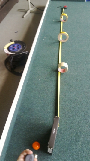
Camera and image processing are crucial components of a successful soccer robot. Consequently, before we could even start to build our robot we had to make sure the camera of the N9 won’t bring any unexpected surprises. In particular, the important questions were:
- Is the angle of view of the camera reasonably wide? Can we position the camera to see the whole field?
- What about camera resolution. If we position a ball at the far end of the field (~5 meters away) will it still be discernible (i.e. at least 3-4 pixels in size)?
- Can it happen that the frames are too blurry when the robot moves?
- At what frame rate is it possible to receive and process frames?
Answering those questions is a matter of several simple checks. Here’s how it went back then.
Resolution and Angle of View
The camera at N9 is capable of providing video at a framerate of about 30Hz with different resolutions, starting from 320×240 up to 1280×720. Among those, there three options which make sense for fast video processing: 320×240, 640×480 and 848×480. The first two are essentially equivalent (one is just twice the size of the other). The third option differs in terms of aspect ratio, and its horizontal and vertical angles of view. The difference is illustrated by the picture below, which shows a measure tape shot from a distance of 10cm.
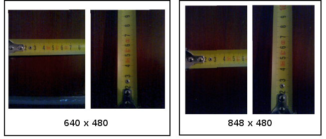
We can see that the resolution 848×480 provides just a slightly larger vertical angle of view than 640×480 (102mm vs 97mm) at the price of significantly reduced horizontal angle of view (65mm vs 86mm). Consequently, we decided to stick with the 640×480 resolution.
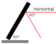
From the picture we can also estimate the angle of view, which is 2*arctan(97/200) ~ 52 degrees vertical and 2*arctan(86/200) ~ 46.5 degrees horizontal. Repeating this crude measurement produced somewhat varying results, with the horizontal angle being as low as 40 and the vertical as large as 60 degrees.
Knowledge that the vertical angle of view is 60 degrees suggested that the phone should also be mounted at around 60 degrees – this provided the full view of the field. As we also needed to see the ball in front of the robot, we had to mount the phone somewhat to the back.
Image Processing Speed
The first code we implemented was just reading camera frames and drawing them on the screen. The code could run nicely at 30 frames per second. Additional simple image operations, such as classifying pixels by colors also worked fine at this rate. Something more complicated and requiring multiple passes over the image, however, could easily drag the framerate down to 20 or 10 fps, hence we knew early on that we had to be careful here. So far it seems that we managed to keep our image processing fast enough to be able to work at 25-30 fps, but this is a topic of a future post.
Camera Speed
One reason why the Playstation 3 Eye camera is popular among Robotex teams is that it can produce 120 frames per second. And it is not the framerate itself, which is important (it is fairly hard to do image processing at this rate even on the fastest CPUs). The important part is that the frames are shot faster and thus do not blur as much when the robot moves. So what about our 30 fps camera? Can it be so blurry as to be impractical? We used our NXT prototype robot (at the time, we did not have our “real” robot, not even as a 3D model) and filmed its view as it drove forward (at 0.4 m/s) or rotated (at about 0.7 revolutions per second). The result is shown below:
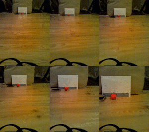
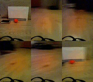
The results are quite enlightening. Firstly, we see that there is no blurring problems with the forward movement. What concerns rotation, however, it is indeed true that even for a moderate rotation speed, anything further away than 50cm or so blurs to be indistinguishable. It is easy to understand, however, that this is not so much a limitation of a 30fps camera but rather a property of rotation itself. At just one revolution per second, objects even a meter away are already flying through the picture frame at 6.28 m/s. Even a 120fps camera won’t help here.
Size of the Ball in Pixels
OK, next question. How large is the ball at different distances? To answer that, we made a number of shots with the ball at different distances from the camera and measured the size of the ball in pixels. The results are the following:
| Distance to ball (mm) | 100 | 200 | 300 | 400 | 500 | 600 | 700 | 800 | 900 | 1000 |
| Ball diameter in pixels (px) | 190 | 105 | 70 | 55 | 45 | 37 | 33 | 29 | 26 | 22 |
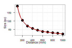
This data can be described fairly well using the following equation (the reasons for this are a topic of a later post):
PixelSize = 23400/(21.5 + DistanceMm)
Two observations are in order here. Firstly, a ball at distance 5m will have a pixel size of about 4.65 pixels, which not too bad. Note that it would be bad, though, if we were to use a resolution of 320×240, as then it would be just 2 pixels. Add some blur or shadows and the ball becomes especially hard to detect. Secondly, and more importantly, if we decide to use such an equation to determine the distance to the ball from its pixel size, we have to expect fairly large errors for balls that are further away than a couple of meters.
So that’s it. Now we’ve got a feel of the camera and ready for actual image processing.
