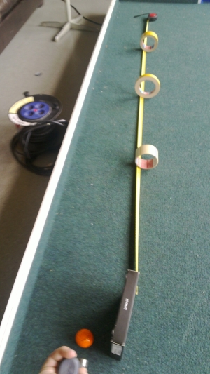
In order to plan the robot (e.g. choose the motors and plan the strength of the coilgun) as well as to implement the simulator, we needed to know the movement dynamics of the golf balls on the field. There is nothing special about their movement – we can safely assume that balls roll with a constant deceleration. The problem is, however, that no one seemed to be able to tell us, even approximately, what this deceleration was exactly.

So we went on and made a crude measurement using the camera, which, in retrospect, is fun to think about. Here’s how it was done.

First, set up a straight path for the ball, marking the 0cm, 50cm, 100cm and 150cm points. We would then roll the ball along this path, measure the time when it passed the four points, and use the obtained numbers to fit the parameters of the equation:

s = v₀ + v(t-t₀) + 0.5a(t-t₀)²

There are three unknowns here (v_0, v, a) – that’s why we need three marks plus the starting mark (t₀) for each measurement (i.e. for each ball run).

Next, we use a camera to film a number of such “ball runs” from the side. Finally, we manually examine the resulting video frames, writing out the time points at which the ball passed each of the marks.

As a side note, if anyone of you, dear readers, for some reason plans on doing something similar at some point of their life, here’s what you should do to find out the timestamps of the frames in a video:

• Install the ffdshow codec. In FFDshow configuration switch on “OSD” (on-screen display) and on the corresponding settings screen put a checkmark near “Frame timestamps”.
• Install Media player classic. In its configuration, switch off all “Internal Filters” and add as “External Filter” the ffdshow Video Decoder. After that, just play the video using this player. You will see frame timestamps and will be able to move frame-by-frame back and forth using the Ctrl+left/right keys.

Obviously, this type of measurement is very crude, however for our purposes it is enough. After having manually “parsed” a video recording of five runs we obtain the following data table:

      T0     T1     T2     T3
1 15.244 15.840 16.598 17.804
2 26.327 26.651 27.100 27.566
3 35.219 35.570 36.020 36.500
4 43.604 44.080 44.638 45.260
5 51.963 52.500 53.182 54.047

The rows here correspond to different runs and the columns – to the four marked points. The values in the cells are timestamps (in seconds from the start of the video).

At last, we fit the movement equation for each row to estimate the “a” parameter. We can do it using R, for example, as follows:

data = data.frame(T0 = c(15.244, 26.327, 35.219, 43.604, 51.963),
                  T1 = c(15.840, 26.651, 35.570, 44.080, 52.500),
                  T2 = c(16.598, 27.100, 36.020, 44.638, 53.182),
                  T3 = c(17.804, 27.566, 36.500, 45.260, 54.047));
for (i in 2:4) data[,i] = data[,i] - data[,1]
data$T0 = NULL
a = c()
for (i in 1:nrow(data)) {
  y = c(0.5, 1.0, 1.5)
  x = t(data[i,])
  x2 = t(data[i,]^2)/2
  m = lm(y~x + x2)
  a = c(a, m$coeff[3])
}

# Median and max a
print(median(a))
print(min(a))

From that we get that the median deceleration of the five runs is  -0.15 m/s² and the smallest estimated value was  -0.25 m/s².

Now we may use this value in the simulator and consider it when choosing the motors.