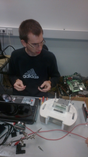
In theory, the dribbler is just a rotating rubber shaft. In practice, making this seemingly simple component is not as trivial as it might seem.
First, we need a metal inner shaft. The ends of the metal shaft must fit perfectly into a couple of ball bearings. There should also be a groove along the length of the shaft to keep rubber in place. As those requirements are fairly specific, it means that the metal shaft has to be lathed manually.
Secondly, we need to pick a suitable type of rubber coating. It must be easily moldable upon the shaft and “sticky” enough to grip the ball. Following the advice of the course supervisors, we used Dragon Skin silicone.
Thirdly, the rubber must be cast onto the metal shaft. This requires preparing three additional components – a properly-sized tube and two caps on it, shaped so that they would hold the shaft right in the middle of the tube. Making the caps meant some more lathe-work for Taavi.
Once the mold is done, the silicone (which comes in two separate components) is mixed, cast into the form onto the shaft, given several hours to harden and taken out of the form, hoping no ugly bubbles or unnecessary objects got caught in it during casting.
Finally, the shaft must be mounted into the ball bearings and geared to a motor (which, in turn, has to be mounted appropriately and connected to a pin of a microcontroller board).
The video below illustrates the functioning of a completed dribbler:
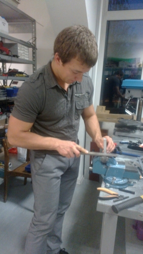
Laser cutting is good for making flat sheets, but not enough to produce 3D shapes. CNC (Computer Numerical Control) milling is the way to make those. As with laser cutting, you can order CNC services at a reasonable price nowadays. It was even easier for our team – Tartu University’s Institute of Technology has a mill available and Taavi knew how to use it.
Piece of a G-code program
The CNC machine is programmed using a special programming language – the G-code, where each instruction corresponds to some movement of the mill. Ironically, despite the obvious practical importance of this language, most programmers or computer scientists have probably never even heard of it. If you are one of them, take a minute to educate yourself and skim through the Wikipedia entry, at least.
Although the CNC code can in principle be generated by CAM systems straight from the 3D CAD-model, it was easier for us to write the program manually, as it allows to account for the specifics of the particular machine in our case.
In the video below, Taavi is running the code he wrote for cutting the coilgun box for the Telliskivi robot:
And if you think this is cool, you might want to take a look at what the expensive industrial CNC mills can do in the hands of expert programmers: (one), (two).
The first Robotex competition took place in 2001. Although I did not take part then, I remember observing with interest the progress of Tartu University teams. Looking back 10 years now, it is fascinating to see how much changed since.
One of this changes is the perhaps wide spread of affordable computerized manufacturing. Laser cutters and CNC milling machines have existed for years now, but it seems that in just the last 10 years has their use become accessible to pretty much anyone who needs it. The more recent 3D printing can’t go without mention – one can get a reasonable tabletop 3D printer at the price of a high-end laptop nowadays.
So for those of you who are new to this thing, here’s a brief example of how things work in the marvellous world where one does not need to know anything about saws and hammers in order to create hard metal objects.
Modeling the part
First, we use a CAD system (SolidWorks, in our case), to create a model of the part. This requires some knowledge of the CAD system, but it is not rocket science, really.
CAD model of a part
Ordering the part
Next, in order to order an actual part from this model, we need to create two files:
As in this particular part we would like the manufacturer to help us with the metal sheet bending, we also need to provide the technical drawing of the final part. The CAD system is quite helpful here too: it takes a couple of clicks to generate the drawing from the model:
Technical drawing
Note that depending on the manufacturer, additional files may be required in certain format as a specification, but in our case this was sufficient. You then send the specification to the manufacturer and wait. Most commercial manufacturers would typically produce parts in batches of at least 100 or so, so if you need just one, you would often have to come up with a personal arrangement.
The price range differs depending on the manufacturer (some have cheaper, less precise machines, some have better ones), chosen material (cutting thinner material requires less power) and personal arrangements. In particular, the total price of computerized manufacturing for the single part shown above, including material (1.5mm aluminium sheet), is less than €20, and can be significantly less, if you manage to get a good deal.
In order to plan the robot (e.g. choose the motors and plan the strength of the coilgun) as well as to implement the simulator, we needed to know the movement dynamics of the golf balls on the field. There is nothing special about their movement – we can safely assume that balls roll with a constant deceleration. The problem is, however, that no one seemed to be able to tell us, even approximately, what this deceleration was exactly.
So we went on and made a crude measurement using the camera, which, in retrospect, is fun to think about. Here’s how it was done.
Measuring ball movement
First, set up a straight path for the ball, marking the 0cm, 50cm, 100cm and 150cm points. We would then roll the ball along this path, measure the time when it passed the four points, and use the obtained numbers to fit the parameters of the equation:
s = v0 + v(t-t0) + 0.5a(t-t0)2
There are three unknowns here (v0, v, a) – that’s why we need three marks plus the starting mark (t0) for each measurement (i.e. for each ball run).
Next, we use a camera to film a number of such “ball runs” from the side. Finally, we manually examine the resulting video frames, writing out the time points at which the ball passed each of the marks.
As a side note, if anyone of you, dear readers, for some reason plans on doing something similar at some point of their life, here’s what you should do to find out the timestamps of the frames in a video:
Install the ffdshow codec. In FFDshow configuration switch on “OSD” (on-screen display) and on the corresponding settings screen put a checkmark near “Frame timestamps”.
Install Media player classic. In its configuration, switch off all “Internal Filters” and add as “External Filter” the ffdshow Video Decoder. After that, just play the video using this player. You will see frame timestamps and will be able to move frame-by-frame back and forth using the Ctrl+left/right keys.
A video frame of a moving ball
Obviously, this type of measurement is very crude, however for our purposes it is enough. After having manually “parsed” a video recording of five runs we obtain the following data table:
The rows here correspond to different runs and the columns – to the four marked points. The values in the cells are timestamps (in seconds from the start of the video).
At last, we fit the movement equation for each row to estimate the “a” parameter. We can do it using R, for example, as follows:
data = data.frame(T0 = c(15.244, 26.327, 35.219, 43.604, 51.963),
                  T1 = c(15.840, 26.651, 35.570, 44.080, 52.500),
                  T2 = c(16.598, 27.100, 36.020, 44.638, 53.182),
                  T3 = c(17.804, 27.566, 36.500, 45.260, 54.047));
for (i in 2:4) data[,i] = data[,i] - data[,1]
data$T0 = NULL
a = c()
for (i in 1:nrow(data)) {
  y = c(0.5, 1.0, 1.5)
  x = t(data[i,])
  x2 = t(data[i,]^2)/2
  m = lm(y~x + x2)
  a = c(a, m$coeff[3])
}

# Median and max a
print(median(a))
print(min(a))
From that we get that the median deceleration of the five runs is -0.15 m/s2 and the smallest estimated value was -0.25 m/s2.
Now we may use this value in the simulator and consider it when choosing the motors.
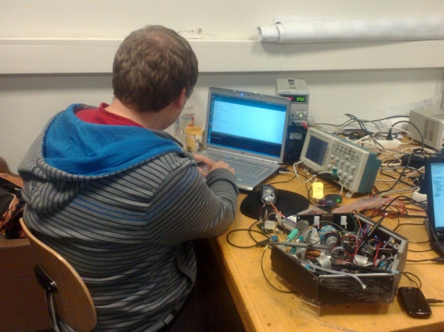
Night or day, there is always someone in the Tartu University’s physics department Digilabor, fiddling with their electromechanical babies. Here are some random shots from one evening when teams Nasty and Sidi were there.
Tõnis, doing brain surgery on the Sidi robot
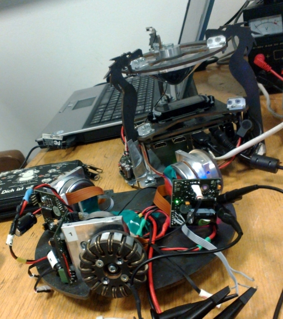
The Sidi robot on the operating table
Harti has taken the Sidi robot’s head off and is up to something
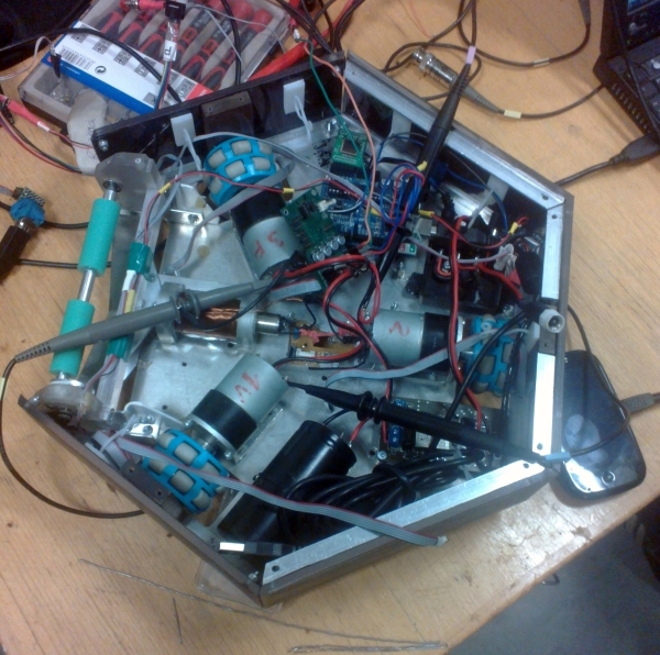
Tartu’s rock star team 18cm-hyperbolic-mirror-custom-omniwheels-CAD-magazine-award team Nasty robot in pieces
Looks like Mihkel has just burned something in the Nasty robot and looks for a replacement
Karl is soldering a motor control PCB for the Nasty robot
Nasty’s motor control PCB rotating a brushless motor with an omniwheel
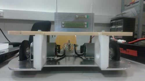
October 15th – we have the second floor’s plate (plastic laser cut by Tööstusplast) and the “tower” for the phone. We do not yet have the “proper” phone mount, but Taavi made a temporary one from whatever he found in the lab, and as a result we have a robot which already looks like the real thing and smells like victory.
The second floor with the “tower”
The first and the second floors together
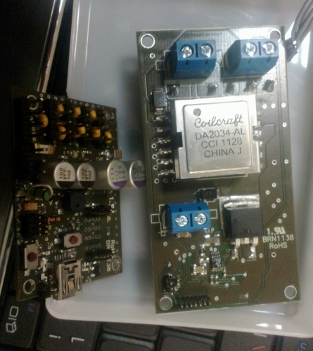
Electronics: The motor-control PCB (left) and the coilgun PCB (right)
It has been approximately a month since the beginning of the project and by that moment we, among other things:
received the aluminium laser-cut base plate for the robot that we ordered from Metec.
received the motors and wheel connectors that we ordered online from Pololu.
made the “preliminary” wheels.
received the parts necessary for the motor control circuit board and soldered them together.
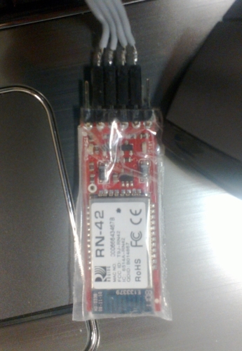
received the Bluetooth module ordered from Proto-PIC.
programmed the motor circuit board to communicate via Bluetooth and drive the motors.
October 10th was the day when we put those things together for the first time and could test the driving. The video below shows the robot base, remote-controlled via Bluetooth using an XBox joystick. Looks fun, doesn’t it?
When we ordered the motors we were afraid they would not be fast enough. Well here they look faster than we need (although this is not even half the final weight of the robot). However, we have some problems, too. Namely, it seems that our motor circuit board cannot handle the motors at low speeds normally. A lot of tuning awaits.
It takes time to design and manufacture the robot’s mechanical parts. It takes time to order, solder together and debug electronics. The third important component of robot development is the main soccer playing algorithm, i.e. the smartphone software, and it is important to start working on it as soon as possible. But how do you go about developing it while the chassis is not available? We used two tricks here.
The simulator
While making the real chassis is time-consuming, making a “virtual one” can take less than a day. So that’s what we actually started with on the very first day of the course – developing a simplistic software simulator, emulating a two-wheeled robot on a football field. The robot can “sense” the balls on the field as well as the opponent’s goal using a simulated camera. It can move around by setting the speed of its two wheels.
Telliskivi Simulator
Such a simulated robot makes it possible to write a soccer-playing control algorithm, not unlike the one we shall be using on the real machine. The control algorithm can connect to this simulated robot via TCP/IP and send commands such as “wheels <a> <b>” (set wheel speeds). This is equivalent to the smartphone connecting to the chassis via Bluetooth and sending the same “wheels” command.
The simulator is written in Python, and the core of it is about 350 lines of code, including comments and doctests. The code is hosted on github here, and everyone is welcome to use it and contribute. It is fairly easy to add custom robot models to it, and in fact, on one of the practice sessions we managed to have a small simulated soccer match against Team Spirit. We lost, because of our attempts to introduce last-minute changes to our algorithm, which happened to break it completely. Thus, the simulator managed to simulate an actual emergency at a competition.
We would like to believe that our simulator was at least in part what motivated Team Spirit to take a go at simulator development themselves, and end up with a way more sophisticated piece of software with better physics engine (JBox2d), better visualization facilities and perhaps better modularity (albeit a more complicated architecture). It is also freely available from github, take a look.
The NXT prototype
Lego NXT prototype
The second trick that has been enormously helpful in the first steps of software development was to take a Lego NXT constructor kit, and hack up a two-wheeler with a simple camera mount. In fact, it was enough to take the “default” NXT robot, turn the position of the NXT brick around, and connect a couple of blocks on top of it for holding the phone.
The NXT brick can be controlled via Bluetooth. The protocol does not seem to be documented anywhere, but some peeks into the source code of the nxt-python package helped to decipher it. Thus way before the mechanics and electronics of the actual Telliskivi robot were ready, we got the opportunity to work on the smartphone code: establishing the Bluetooth connection, checking connection latency and getting the first attempts at ball detection from a camera mounted on an actual moving robot.
In fact, the N9-controlled NXT is a rather fun toy in itself!